How I matched 10 million messy business records to 1.7 million companies
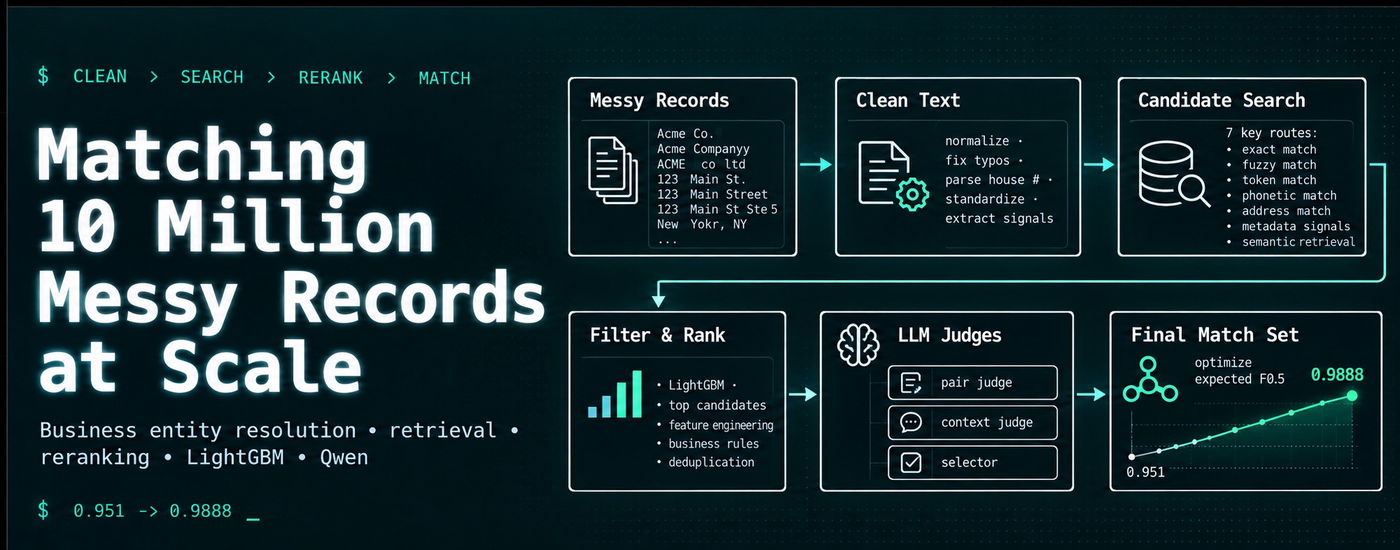
The problem was business entity resolution, set as a large-scale ML competition.
- The data: a clean list of 1.73 million businesses, plus about 10 million messy records from two other sources.
- The task: for every business, find all the messy records that are really that business.
- The metric: macro F0.5, averaged per business. It counts precision twice as much as recall, so one wrong match costs about four times as much as one missed match.
My final leaderboard score was 0.9888. This post is the whole pipeline that got there, and the steps along the way that moved the score.
What the data looked like
Every business in the clean list shows up again in the other two sources as damaged copies:
- Names had typos, letters replaced by look-alike digits (
5terling), reordered words, legal forms moved or dropped (LLC,Pvt Ltd), and sometimes a website instead of a name. - Addresses were upper-cased, abbreviated (
RD,BLVD), missing a house-number digit, or missing entirely.
On top of that, the data contained decoys: records built to look like a real business but belonging to none. A decoy might add one business word ("Holdings"), shift the house number by a few, or change the legal form.
Two more things shaped everything I built:
- A messy record belongs to at most one business. So I searched from the record's side: for each record, pick its best business or none.
- The test set had a country the training data never had. Training covered India and the US. The test added France, with no labels at all.
The final pipeline
The core idea is a retrieve-then-rerank cascade: cheap tools look at everything, expensive tools only look at what's left. Each stage narrows the list so the next, slower and smarter stage can afford to read it carefully.
 Clean list (1.73M businesses) + messy records (~10M)
                         │
                         ▼
 ┌──────────────────────────────────────────────────┐
 │ 1. NORMALISE TEXT                   rules, CPU   │
 │ make messy and clean text look alike             │
 └──────────────────────────────────────────────────┘
                         │
                         ▼
 ┌──────────────────────────────────────────────────┐
 │ 2. CANDIDATE GENERATION (blocking)               │
 │ inverted index top 40  +  bge-m3 top 10          │
 │ (top 30 if no address)  -> ~40-70 per record     │
 └──────────────────────────────────────────────────┘
                         │
                         ▼
 ┌──────────────────────────────────────────────────┐
 │ 3. FILTER + GROUP CHECK            LightGBM, CPU │
 │ score every candidate, keep the top 3            │
 └──────────────────────────────────────────────────┘
                         │
          ┌──────────────┼──────────────────┐
          ▼              ▼                  ▼
 ┌──────────────┐ ┌───────────────┐ ┌────────────────────┐
 │ PAIR JUDGE   │ │ CONTEXT JUDGE │ │ QWEN SELECTOR      │
 │ cross-encoder│ │ cross-encoder │ │ listwise LLM,      │
 │ record +     │ │ + other copies│ │ hard records only: │
 │ business     │ │ + rivals      │ │ 1 of top 5 or none │
 └──────────────┘ └───────────────┘ └────────────────────┘
          └──────────────┼──────────────────┘    GPU
                         ▼
 ┌──────────────────────────────────────────────────┐
 │ 4. STACKER (combiner)              LightGBM, CPU │
 │ learn which judge to trust when                  │
 └──────────────────────────────────────────────────┘
                         │
                         ▼
 ┌──────────────────────────────────────────────────┐
 │ 5. CALIBRATE + DECIDE PER BUSINESS         math  │
 │ keep the records that maximise expected F0.5     │
 └──────────────────────────────────────────────────┘
                         │
                         ▼
                 matching_results.tsv
I'll follow one record through every step:
 biz_101  Sterling Traders Pvt Ltd  | 12 MG Road, Pune     <- the real business
 biz_102  Sterling Holdings Pvt Ltd | 14 MG Road, Pune     <- a near-identical neighbour

 rec_9    5TERLING TRADERS PRIVATE LIMITED | 12 M.G. RD, PUNE    <- which one is it?
1. Normalisation: make both sides comparable
No model here, just deterministic Python rules running on CPU in parallel with multiprocessing. They undo the damage
so the same business looks the same on both sides:
 5TERLING TRADERS PRIVATE LIMITED | 12 M.G. RD, PUNE
   -> name "sterling traders"   legal form "pvt"   address "12 mg road pune"   house no. "12"
- Leetspeak repair: digits used as letters are swapped back:
5terling→sterling. - Legal-form extraction: "Pvt Ltd" and "Private Limited" both become the code
pvtin their own field, so they stop looking like a difference in the name. - Abbreviation expansion:
RD→road,BLVD→boulevard. - Primary house number: pulled out on its own, because it's the strongest clue against decoys.
- Transliteration: Indian-script names are converted with a dictionary learned from the training matches.
Copies were word-for-word transliterations, so pairing words by position gives "सूर्य → surya". Anything left goes
through
anyascii, which converts letter by letter. - Phonetic codes: Metaphone and NYSIIS turn each word into a sound code, so "Sterling" and "Stirling" get the same key.
2. Candidate generation: from 1.73M businesses to a short list
Comparing every record with every business means 10M × 1.73M ≈ 17 trillion pairs. That's years of compute. So first, a step called blocking finds a short list of businesses that might match.
Inverted index. This works like the index at the back of a book: instead of "page → words", it stores
"word → businesses that contain it". For rec_9, look up its words and collect every business that shares one.
Each shared key is weighted by IDF (inverse document frequency, log(total businesses / businesses with this
key)): a rare word like "sterling" is strong evidence, while a common word like "traders" is weak. There are seven
key types: words, word pairs, house number + street, character 4-grams for typos, and phonetic codes for spelling
variants. In code, it's a polars join on hashed keys, not a Python dictionary, which is much faster at this scale.
Dense retrieval with bge-m3. The index fails when a copy shares almost no words with its business (heavy typos, reordering, another script). bge-m3 is a multilingual embedding model: it turns any text into a vector of 1,024 numbers, like coordinates for meaning. Texts that mean the same land close together, measured by cosine similarity.
Out of the box, it puts "Sterling Traders" and "Sterling Holdings" very close, which is exactly the decoy trap. So I fine-tuned it on triplets, using a contrastive loss: pull the record and its true business together, and push away a hard negative (the wrong business the index ranked highest):
 anchor:     5TERLING TRADERS PRIVATE LIMITED | 12 M.G. RD
 positive:   Sterling Traders Pvt Ltd | 12 MG Road          (pull closer)
 negative:   Sterling Holdings Pvt Ltd | 14 MG Road         (push away)
The other 255 businesses in each training batch act as extra negatives for free (in-batch negatives). For the search itself, every business and record is encoded, and the nearest 30 businesses are found with one matrix multiply on the GPU. That's an exact search, with no approximate index.
Merge. The two lists are joined, with duplicates removed: the top 40 from the index plus the top 10 from bge-m3 (30 for records with no address, where the index is weakest). Each pair keeps both search scores and a flag saying which search found it. Together the two searches reach about 99% recall: the true business is on the list 99% of the time. From here on, the job is to pick the right one, or none.
3. The filter: score the short list cheaply
The search is tuned for recall, not ranking. "Sterling Holdings" scores high on both searches because the words and meaning are close. The filter is a LightGBM model, a gradient-boosted decision tree ensemble: hundreds of small yes/no trees, each one learning to fix the mistakes of the trees before it. It works on tabular numbers, so each pair becomes 65 features, and it outputs a probability:
 NAME            fuzzy string similarity (Levenshtein ratio, token-set, Jaro-Winkler), exact squashed match
 ADDRESS         same fuzzy measures, is it missing?
 HOUSE NUMBER    equal? log of the difference? one a suffix of the other?
 LEGAL FORM      same, conflicting, or missing?
 SEARCH          IDF score per index route, bge-m3 similarity and rank, found by both?
 RANK            is this the record's best candidate? gap to the best?
 CROWDING        how many near-identical names compete for this record?
 rec_9 -> biz_101  0.97   same name, same number, same legal form, rank 1
 rec_9 -> biz_102  0.08   different number, "Holdings" vs "Traders"
The rank and crowding features matter most. A decoy can score well on its own, but it rarely beats the real copy among its rivals.
Group check. A second LightGBM compares the record with the business's other copies, not just the clean entry. A copy with no address looks weak on its own, but it usually looks like its siblings.
Only the top 3 per record move on, about 7.8M pairs on the test set, so the slow GPU models never waste time on obvious non-matches.
4. Three judges: read the hard cases carefully
The filter only sees numbers. The judges read the actual text, and each one sees something the others can't:
| Judge | Type | What it reads | What it catches |
|---|---|---|---|
| Pair judge (bge-reranker-v2-m3) | cross-encoder | the record and the business, together | wording: "Traders" ≠ "Holdings", 12 ≠ 14 |
| Context judge (same model, trained separately) | cross-encoder | the pair, plus the business's other copies and the record's rivals | weak copies that match their siblings |
| Qwen selector (Qwen3-4B + LoRA) | listwise LLM | a hard record and its top 5 businesses, side by side | decoy twins, and "none of these" |
Cross-encoder vs embedding. bge-m3 encodes each text separately, which is fast enough to search millions. A cross-encoder reads both texts together in one pass, so every word of the record can be compared with every word of the business. It's far more accurate, and far too slow for anything but a short list.
Listwise selection. A pairwise judge scores one pair at a time and never sees the twin. Qwen gets a multiple-choice question:
 Record: 5TERLING TRADERS PRIVATE LIMITED | 12 M.G. RD, PUNE
 A) Sterling Traders Pvt Ltd  | 12 MG Road
 B) Sterling Holdings Pvt Ltd | 14 MG Road
 C) ...
 F) none of these
 Answer: A
The options are shuffled, so the position carries no information. LoRA (low-rank adaptation) keeps Qwen's 4B weights frozen and trains only a small add-on, so fine-tuning fit on one H100 in under an hour. Qwen only reads "hard" records, where the filter was unsure or a rival came close: about 785k test records, not 10 million.
5. Stacker, calibration and decision: one answer per business
Stacking. Each pair now has several opinions. A LightGBM stacker takes the filter score, the three judge scores and 15 pair features, and learns when to trust which judge. For example: no address → lean on the context judge; two near-identical rivals → lean on Qwen. The output is one probability per pair.
Calibration. A model saying 0.9 should be right 90% of the time. I fitted a correction curve on held-out data, with a separate one for records with no address, so the probabilities could be trusted in the next step.
Expected-F0.5 decision. There's no single threshold. For each business, sort its records by probability and keep the prefix that gives the best expected F0.5. Since a wrong match costs about four times a miss, it leans toward leaving uncertain records out. If nothing is likely, the business gets an empty list, which is the right answer for businesses that have no copies.
 biz_101 -> rec_5 0.99, rec_6 0.98, rec_9 0.96, rec_80 0.20     keep the first three
 biz_102 -> nothing likely                                      empty, correctly
Cross-fitting. Every model was trained twice, each time on one half of the businesses, and each copy only scored the half it never saw. This gives out-of-fold scores. Without it, the stacker would learn from scores on memorised data, which look far more confident than anything it would see on the test set.
How the training was done
Every step was cross-fitted, as described above. I split the training businesses into two halves; each model was trained on one half and scored the other. That way the next stage always learned from honest, out-of-fold scores. On the test set, both copies score every pair.
The work split cleanly into CPU jobs and GPU jobs.
 CPU  (AWS r7i.48xlarge: 192 vCPUs, 1.5 TB RAM)
   cleaning ──► word-key search ──► 65 features ──► LightGBM filter ──► group check ──► combiner
                                                        ▲                                  ▲
 GPU  (H100s on Modal, L4s on AWS, earlier RunPod)      │                                  │
   bge-m3 fine-tune ──► meaning search ──────────────────┘                                  │
   reranker x2 + context judge x2 ─────────────────────────────────────────────────────────┤
   Qwen3-4B selector (train on H100, score on 4x L4) ───────────────────────────────────────┘
CPU: everything LightGBM
LightGBM doesn't need a GPU. All the tree models ran on one 192-core machine with 1.5 TB of RAM, because the feature tables were large: the training features alone were about 30 GB.
| Job | Data | Settings | Time |
|---|---|---|---|
| Text cleaning + word-key search | ~10M records per split, 7 key routes | parallel over 180 cores | tens of minutes per split |
| Filter (LightGBM) | every training record × its top 40 candidates, with 25% of the easy negatives kept | learning rate 0.1, up to 3,000 rounds, early stopping | the largest CPU job, about an hour |
| Group check (LightGBM) | each record's top candidates + its business's confident copies | cross-fitted | minutes |
| Combiner (2 × LightGBM) | about 2.6M judged pairs per half | 800 rounds, 63 leaves | about 12 minutes per full run |
GPU: the language models
| Model | What it learned from | Hardware | Time |
|---|---|---|---|
| bge-m3 (meaning search) | triplets of record, true business, hardest wrong business | H100 | a few hours, then exact search as a matrix multiply on the GPU |
| bge-reranker-v2-m3, pair judge (2 copies) | judged pairs from one half of the businesses each | H100 | about an hour per copy |
| bge-reranker-v2-m3, context judge (2 copies) | the same pairs, with each business's other copies and rival businesses in the text | H100 | about an hour per copy |
| Qwen3-4B + LoRA, selector | 180k hard records, each shown with its top 5 businesses | 1 × H100 | about 53 minutes (~41 examples per second) |
| Selector scoring | 785k hard test records | 4 × L4 | about 3.5 hours |
Two details made the GPU budget work:
- Only the hard cases get the expensive models. The filter keeps each record's top 3 businesses (7.8M pairs out of about 200M candidates), and the Qwen selector only reads records the filter is unsure about.
- Parallel, short-lived GPUs. Training jobs ran as containers on Modal, up to 10 H100s at a time, and shut down when finished. A late experiment with a 7B selector trained in 13 minutes on 8 H100s and scored everything in about 15 minutes on 10.
The early versions ran on smaller hardware. The first LightGBM models trained on 64-core Azure VMs. The first Qwen judge, the one behind the 0.951 to 0.973 jump, and the first embedding runs used RunPod GPUs (an L40, then an H100). I moved to the big AWS machine and to Modal once the data and the number of models grew.
The journey: what actually moved the score
| Step | Leaderboard |
|---|---|
| LightGBM with string features, a fixed threshold | 0.951 |
| + a Qwen LLM judge on the unsure pairs | 0.973 |
| + full data, 7 search routes, bigger LightGBM | 0.979 |
| + reranker, meaning search, context judge, combiner | 0.986 |
| + pair features, an F0.5-optimal decision rule | 0.9879 |
| + Qwen3-4B selector, decisions retuned on a better held-out | 0.9888 |
The Qwen moment
The biggest single jump came from adding an LLM judge. My first LightGBM sat at 0.951. Adding a Qwen model to re-judge only the pairs LightGBM was unsure about took it to 0.973 in one step. It worked again on the bigger pipeline: 0.968 without the judge, 0.979 with it.
String features can say that two names share 80% of their letters. They can't say that "Nayak Traders Pvt Ltd" and "NAYAK TRADING PRIVATE LIMITED" are the same shop, while "Nayak Holdings" next door is not. A language model can.
I also learned the limits:
- Judges give the most when the base is weak. By the end, adding a bigger Qwen judge to an already strong stack moved the local score by only +0.0002.
- Bigger wasn't automatically better. I trained a 7B selector late in the competition. It agreed with the 4B almost everywhere, because the combiner already knew what the bigger model knew.
The held-out that lied
For a while my local validation said every change was a gain, and the leaderboard disagreed. The cause was a shortcut in how I built the held-out:
- I scored a 35% sample of records, so many wrong matches pointed at businesses outside the sample and cost nothing.
- The sample had half the test set's density of decoys.
So tweaks that added matches looked free locally and cost points on the test. Once I rebuilt the held-out to look like the test (every business, the full truth, decoys added to match the test's density), three of my "improvements" turned out to be losses: an address-less boost, a model ensemble and a joint decoder. Removing them gave the final gain.
What I'd do differently
- Find the score gap first. India and the US were already strong, while France (15% of the test, no labels) was where most of the remaining loss sat. I spent too long polishing the part I could measure.
- Use leaderboard uploads as experiments early. For a segment with no labels, two uploads that differ only in that segment, one stricter and one looser, tell you more than any amount of local reasoning.
- Make the local eval look like the test before tuning anything. Every decision tuned on a biased held-out has to be tuned again.
The stack
| Model | Size | Licence | Role |
|---|---|---|---|
| BAAI/bge-m3 (fine-tuned) | 568M | MIT | meaning search |
| BAAI/bge-reranker-v2-m3 (fine-tuned) | 568M | Apache-2.0 | pair judge, context judge |
| Qwen3-4B + LoRA | 4.0B | Apache-2.0 | selector |
| LightGBM | n/a | MIT | filter, group check, combiner |
Everything was learned from the provided data. Training ran on rented GPUs (H100s on Modal, L4s on AWS), and the LightGBM and data work ran on one large CPU machine.
Final score: 0.9888 macro F0.5.